Two oversized dice rolling into view and settling on a three and a four.
In the previous chapter, we hinted at thinking probabilistically about extreme scores in a distribution. Here, we’ll go into that idea in more detail. We’ll think about what statisticians mean when they talk about probability and how we go about quantifying it. We’ll need to introduce some new terminology, including probability distributions, and then we’ll return to \(z\) scores and see how a normal distribution lets us attach precise probabilities to regions of scores.
A Brief History of Probability
People have been thinking about probability for a long time, at least in a broad sense. It’s a useful thing to be able to make predictions about an uncertain future. Can I kill this sabre-toothed tiger, or will it probably kill me first? How much crop should we plant to feed the group? For most of that history, there were no formal ways of articulating how probable something might be. The best people could do was offer rough verbal descriptions. Aristotle distinguished between things that are pretty much unpredictable (“the accidental”), certainties (“that which is always”), and “that which is for the most part”—things that happen with some predictability. “That honey-water is useful for a patient in a fever is true for the most part,” Aristotle wrote as an example (Aristotle, n.d., Book VI, sec. 2). Sometimes it might help, sometimes not: it’s not certain, but neither is it entirely unpredictable. It’s something in between, more or less probable.
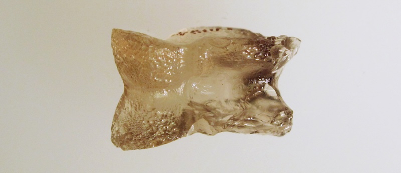
But how much more or less? The idea of representing uncertainty with numbers and reasoning about it mathematically was a relatively recent development. One of the early inspirations came not from life-and-death decisions but from games of chance. For thousands of years people have been playing games using bits of animal bone—two-sided, coin-like worked and decorated pieces of bone, or astragali, the four-sided ankle bones of sheep and goats. Games played this way were so popular that some people even manufactured astragali out of clay, stone or glass.
According to the card describing this glass astragal at the Metropolitan Museum of Art in New York, playing with them was so much fun that “knucklebones have been found in tombs where they must have been intended to help the deceased while away endless time.” (So I guess, in a way, it was a matter of life and death.)
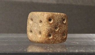
Astragali have four faces stable enough to land on, but the faces aren’t the same size or shape, so the four results aren’t equally likely. Cubical dice offered a more regular alternative to the irregular animal bones. The example below, something like 4,000 years old, even has the convention of opposite sides adding to seven that modern dice follow. These regularly shaped dice proved appealing to gamblers, and eventually to mathematicians, because it meant they could count outcomes and reason about them in a consistent way.
Figure 6.2: Terracotta die, Mohenjo-daro, c. 2500–1900 BCE. Ashmolean Museum, EAMd.25. Photograph by Zunkir, CC BY-SA 4.0.
Catan
To see how this kind of probabilistic thinking works, let’s think about a relatively recent game, Catan. It’s a board game played by rolling a pair of dice (not goat knucklebones, thankfully). The board consists of hexagonal terrain tiles, each producing a resource such as wood or grain. Resources are good, so you want to get as many as possible. (We’ll ignore the differences between resources and other complications of the game.)
Most tiles have a number token. Players can place settlements at the corners where tiles meet. Then every time the dice are rolled, if the sum of the two dice matches the number on a tile touching your settlement, it’s payday—you get that resource. So choosing where to settle means choosing which sums will pay you for the rest of the game. Suppose you get to go first, and you just want the greatest chance of getting something on each roll. Where would you settle? Why?
Choose a settlement
0 of 2
1
Choose a corner to give yourself the best chance of getting
resources. No need to calculate anything yet, just go with your gut.
Click a corner to place your settlement; your choice is saved
automatically.
A simplified Catan board. Settlements go at the corners where numbered
tiles meet; a matching dice total makes a tile produce a resource.
Enable JavaScript to choose a corner.
2
Place your settlement by clicking a spot on the board above, then
explain your choice here in a few words.
Explanation
Keep your reasoning in mind as we work through the dice example. You
will be able to compare your initial choice with what the probabilities
suggest.
Defining Probability
Let’s lay out some technical terms now, so that we have the precise language we need to reason about whether you picked the best spot.
First, what exactly do we mean by probability? As you might expect, there are distinct schools of thought and intense disagreement, which I am happy to sidestep for the most part. In this book, we will take an approach based in the frequentist tradition, since it’s the one that has dominated the social sciences for most of their history. A probability, in the frequentist sense, is a number that describes what would happen if we could repeat something many times: the proportion of repetitions in which some event of interest would occur in the long run. Probabilities range from 0 to 1. A probability of .5 means that, in the long run, we would expect the event to occur about half the time.
Let’s think about some simple situations in which there are a small number of equally-likely outcomes that we can count. (Later, we’ll generalize the same ideas to situations where outcomes are not equally likely, and to continuous variables and models where counting individual outcomes no longer works.) We’ll need some terms:
An outcome is one elementary result of a chance process.
An event is the outcome or collection of outcomes we’re actually interested in.
The sample space is the set of all the possible outcomes.
We use a capital letter \(P\) to denote probability and put the event we’re interested in inside parentheses. So \(P(A)\) means the probability of Event A. When every outcome in the sample space is equally likely, we can find that probability by counting the outcomes in A and dividing by the total number of possible outcomes.
\[ P(A) = \frac{\text{number of outcomes in } A}{\text{total number of possible outcomes}} \]
If you flip a fair coin, for example, there are two possible outcomes, heads or tails. The entire sample space consists of those two outcomes. If we want to denote the probability of heads, one of those two equally likely outcomes, we would write \(P(\text{heads}) = 1/2 = .5\). (Effectively the event is the outcome; there’s only one outcome that gets you heads.) Likewise, we would write the probability of tails as \(P(\text{tails}) = 1/2 = .5\).
Similarly, if we roll a fair six-sided die, there are six equally likely outcomes in the sample space, the die’s faces, one through six. So the probability of rolling a six is \(P(6) = 1/6 \approx .17\).
Perhaps we’re interested in the event of rolling an even number on a single six-sided die. Now we have an event that can be produced by more than one outcome. There are three individual outcomes (2, 4, 6) that would constitute that event. So the probability of rolling an even number is \(P(\text{even}) = 3/6 = 1/2 = .5\).
Rolling Two Dice
The same logic applies to rolling multiple dice; the sample space just expands, and we have to be careful about how to count things. Something that tripped up some early gamblers is that we’re interested in the sum of the dice, like the probability of rolling a 7, but some sums can be arrived at in multiple ways.1 Did you notice the red and blue dice at the top of the chapter? Red landed on 3 and blue landed on 4, for a sum of 7. But what if red had instead landed on 4 and blue on 3? The total would have been 7 as well. We need to count all the different ways each die might land to give the various possible totals.
Assuming both dice are fair and neither die’s result affects the other’s, each of the six red results can be paired with each of the six blue results, giving \(6 \times 6 = 36\) equally likely outcomes. Table 6.1 shows them all: rows give the red die’s result; columns give the blue die’s result.
Table 6.1: The totals associated with all 36 ordered outcomes of rolling two dice.
1
2
3
4
5
6
1
2
3
4
5
6
7
2
3
4
5
6
7
8
3
4
5
6
7
8
9
4
5
6
7
8
9
10
5
6
7
8
9
10
11
6
7
8
9
10
11
12
We can take the 36 sums in the table and draw a bar graph counting how often each value appears. Each bar in Figure 6.3 counts the entries in the table that give that total. A total of 2 appears only once, for example, while 7 appears six times.
Figure 6.3: Counts of the dice totals in the table of 36 possible outcomes.
Bar graph of counts among 36 possible ordered dice outcomes. Totals 2 through 12 have counts 1, 2, 3, 4, 5, 6, 5, 4, 3, 2, and 1.
Now let’s make a similar version of the graph, with a small mathematical change:
Figure 6.4: The same dice totals, with each count divided by 36 to give a probability.
Bar graph showing probabilities for the sum of two dice, rising from 1/36 for 2 to 6/36 for 7, then falling symmetrically to 1/36 for 12.
Did you notice the difference? We divided each count by the total, 36, to turn frequencies into proportions. The shape of the distribution is the same; only the vertical scale changes.
It’s a small mathematical tweak but a bigger conceptual leap. Rather than counting every outcome in the sample space once, as in Figure 6.3, each bar tells us the long-run proportion of future rolls on which that total would occur. These probabilities form a probability distribution. It shows every possible value of the variable and the probability attached to each one. The counts in Figure 6.3 add up to 36; the probabilities in Figure 6.4 add up to 1.
We can use it to predict frequencies: over 100 rolls, for example, we’d expect a total of 7 about \(100 \times (6/36) \approx 17\) times. (If we actually roll the dice 100 times we might not get exactly that many sevens; we’re describing what to expect from the chance process, not a strict guarantee. More on this a little later.)
One more thing to note. If we’re interested in two or more mutually exclusive events, meaning they cannot happen together on the same roll, we can add their probabilities to find the probability of one or the other. For example, the probability of rolling a sum of 5 or 6 is:
Using the table of 36 equally likely outcomes, what is the
probability of rolling a sum of 9? Enter a decimal, rounded to at least
two decimal places.
Hint
Count the cells containing a 9. Remember that a 4 on the first die
and a 5 on the second is a different outcome from a 5 on the first die
and a 4 on the second.
Answer
0.1111
Explanation
There are four ways to make a 9 — (3,6), (4,5), (5,4), and (6,3) —
out of 36 equally likely outcomes, so \(P(9) =
4/36 \approx .11\).
2
The Catan board earlier had an intersection that touches tiles
numbered 3, 8, and 10. What is the probability that it earns resources
on a given roll? Enter a decimal, rounded to at least two decimal
places.
Hint
A single roll cannot be two different sums at once, so no outcome
gets counted twice. Add up the ways.
Answer
0.2778
Explanation
There are two ways to roll a 3, five ways to roll an 8, and three
ways to roll a 10, and no outcome is more than one of them, so \(P(3 \text{ or } 8 \text{ or } 10) = (2 + 5 + 3)/36
= 10/36 \approx .28\).
Back to Catan
Now we can return to your settlement in Catan. Armed with the tools and terms we just outlined, are you still pleased with your choice?
Figure 6.5: The Catan board, with the probability that each intersection earns at least one resource on a roll indicated by the size and color of each potential settlement: bigger, greener markers have higher probabilities. If you chose a corner earlier, it is circled, and the board’s best corner is marked.
The Catan board with corners rated by their probability of producing at least one resource. The best corner touches 5, 6, and 9, with probability 13/36.
We can definitively answer the question of which corner is best. On this board it’s where the 5, the 6 and the 9 meet, up near the top. It pays out if the total is any one of those numbers. Since those events are mutually exclusive, we can add:
Nothing else on this board gets past \(10/36\), or about .28. The board had some clues: the red numbers, the 6s and 8s, are individually the most likely totals (since there’s no 7 on this board; in the real game something else happens when 7 is rolled). But a settlement’s probability depends on all the different totals that pay it. The little dots on the tokens were another clue: they count how many of the 36 outcomes produce that total. To find the probability of any intersection on this board, add the dots on the tiles it touches and divide by 36.
Of course, just picking the best spot in a statistical sense won’t win you the game. Like we pointed out already, a probability of about \(.36\) does not guarantee that those three numbers will occur on exactly 36 out of 100 real rolls. In a single game of Catan, any given corner might pay out more or less than expected.2 But at least now you can reason about your choice in a precise way.
Probability and Distributions of Scores
The same logic applies to the scores we study in social science. We can ask for the probability of randomly selecting a score equal to a value, above a value, or within a range.
Take this little distribution of ten scores.
Figure 6.6: A block histogram showing a distribution of 10 scores: four 1s, three 2s, two 4s, and one 5.
Block histogram of ten scores: four 1s, three 2s, two 4s, and one 5.
If we select one score at random, each of the ten blocks is one equally likely outcome. Let \(X\) stand for the value of the score we select. Four of the ten blocks have a value of 1, so:
\[ P(X = 1) = \frac{4}{10} = .4 \]
There are no blocks at 3, so \(P(X=3)=0\). And we can define events that collect several values at once:
\[ P(X \ge 4) = \frac{3}{10} = .3 \]
\[ P(1 < X < 5) = \frac{5}{10} = .5 \]
The block histogram describes scores we’ve already observed, but those proportions also tell us what to expect when we randomly select one of the blocks. If we repeatedly select a block at random, putting it back each time, we would expect about 40% of our selections to give a score of 1. Once again, we’re using a distribution to reason about selections we haven’t made yet.
What if we’re interested in a continuous variable, such as height or reaction time, rather than a little collection of scores we can count? Remember the smooth curves in Chapter 2. They represented models of how scores were distributed, including scores we hadn’t actually observed. We called the height density back in Chapter 2. A high part of the curve means scores are concentrated around that value, but the density itself isn’t a probability. We scale the curve so that its total area is 1. Computing the area between two scores then gives the probability of a randomly selected score falling within that interval.3
Figure 6.7: A smoothed curve like the ones we saw in Chapter 2. The shaded region between scores of 2 and 3 contains about 30% of the total area.
A smooth density curve with the region between scores of 2 and 3 shaded, containing about 30% of the total area.
For the curve in Figure 6.7, which you might recognize from Chapter 2, about 30% of its area lies between 2 and 3. That means a randomly selected score from that modeled distribution has about a .30 probability of falling within that range. Of course, the math behind that answer depends on the precise contours of that curve: a different shape would produce different probabilities. That’s why I mentioned back in Chapter 2 that one curve in particular would become very important to us: the normal curve.
The Normal Distribution
The normal distribution is so useful to us because its entire shape is determined by just two numbers: the mean and the standard deviation. Those two features are enough to determine probabilities under a normal model.
Figure 6.8: A normal curve, representing a simple model of a population of scores.
A symmetrical bell-shaped normal curve representing a hypothetical population of scores.
Okay, the math that defines the curve is more involved than I’m making it sound. Here’s the equation:
You don’t really have to know this equation for the work we’re going to do throughout this book, so if it makes you sweat just looking at it, don’t worry. But it is worth looking at briefly to get a sense of how it’s constructed. The value \(Y\) gives the height of the curve (its density) at a particular value of \(X\) (which is part of the exponent over to the right). You can find both the parameters, \(\mu\) and \(\sigma\), along with some other constants like \(e\) and \(\pi\). But again, don’t worry about remembering the specifics. Just know that the equation defines the curve precisely, its shape is entirely determined by the mean and standard deviation, and it gives us a curve with a total area of 1, so we can read its areas as probabilities in exactly the way we just described.
Continuing with the historical theme of games of chance, this was figured out in large part by French mathematician Abraham de Moivre, while thinking about the long-run probabilities of simple events with two equally-likely outcomes, like a coin toss. Like we saw earlier, for a fair coin, each outcome (heads or tails) has a probability of \(.5\). But what happens when you toss a coin a bunch of times, say 3,600? Will you get precisely half—1,800—come up heads? Probably not. Toss the coin another 3,600 times and you’ll get a different answer again. If you had the time to do this over and over again, the answers would usually be somewhere close to the expected 1,800; occasionally (but rarely) would it be far away.
De Moivre realized that we can approximate the distribution of all these possible outcomes with a simple smooth curve—the normal distribution. He calculated that the distribution was centered at 1,800 and had a spread equivalent to what we would now call a standard deviation of 30. Using his normal curve, De Moivre worked out that if we were to flip a coin 3,600 times, there was about a 68% chance of getting between 1,770 and 1,830 heads (Moivre, 1738, Corollary 4). In other words, .68 of the area under the curve is in the region between those values.
Figure 6.9: A normal approximation for the number of heads in 3,600 fair coin flips. The shaded region, from 1,770 to 1,830 heads, contains about 68% of the total area.
Normal approximation for the number of heads in 3,600 fair coin flips, with mean 1,800 and standard deviation 30. The shaded region from 1,770 to 1,830 contains about 68% of the area.
The Unit Normal Table
This math works for a normal distribution with any mean and standard deviation, but it is often easiest to work with the standard normal distribution, also called the unit normal distribution. This is a normal distribution with a mean of 0 and a standard deviation of 1. Sound familiar? We described standardizing distributions using \(z\)-scores in exactly this way in Chapter 5. For a normally distributed variable, that transformation gives us this standard normal distribution.
So now we can determine areas under the curve and interpret them as the probability of a randomly selected score falling in that region. So, for example, 34.13% of the area of the curve lies between the mean and one standard deviation above the mean. Because it’s symmetrical, the same 34.13% lies between the mean and one standard deviation below the mean. Another 13.59% lies between one and two standard deviations from the mean on each side. And 2.28% lies more than two standard deviations above the mean, with another 2.28% more than two standard deviations below it. Together, the two extreme regions contain about 4.56% of the distribution.
Figure 6.10: Percentages of the standard normal distribution in each region between \(z=-2\), \(z=-1\), \(z=0\), \(z=1\), and \(z=2\).
Standard normal curve divided at z = -2, -1, 0, 1, and 2, with each region labeled by the percentage of the distribution it contains: 2.28%, 13.59%, 34.13%, 34.13%, 13.59%, and 2.28%.
Of course, we aren’t limited to whole-number \(z\)-scores. We can take any\(z\)-score and determine the probability of a score falling above or below that value under a standard normal model. In the olden days, you would look up something called a \(z\) table, a standard normal table, or a unit normal table. (Computers have made these tables largely obsolete, but it’s useful for us to see how they work, because whatever statistical software you might use in practice is applying the same logic and math.) These tables vary in how they’re arranged. The one below lists nonnegative \(z\) scores along with the areas to their left, to their right, and between the mean and the score.
Table 6.2: The unit normal table, showing areas to the left, right, and between the mean and a given \(z\) score. Scroll to see more values.
Unit normal table showing areas to the left, right, and between the mean and z.
So for a \(z\) score of zero, it’s exactly half and half; 50 percent of the distribution lies on either side of zero, because zero is the mean and the distribution is symmetrical. In other words, under a normal model there is a 50 percent chance of observing a score greater than the mean and a 50 percent chance of observing a score lower than the mean.
If we take a \(z\) score of 1, we look for that row in the table. The area to the left of \(z=1\) is about .84, so roughly 84 percent of the distribution lies below it. In percentile language, a score with \(z=1\) is at about the 84th percentile. The area to the right is just under .16, and the area between the mean (where \(z=0\)) and \(z=1\) is .3413, just like we saw before. How about a \(z\) score of negative one? Standard normal tables don’t always list negative \(z\) scores, because the symmetry of the distribution means the relevant areas are the same as for a positive \(z\) score on the opposite side of the mean. Only the direction flips: the smaller area (0.1587) is to the left of \(z = -1\) and the larger area (0.8413) is to its right.
What if we want the area between two scores, such as \(z=0.5\) and \(z=1.5\)? Subtract the area to the left of \(0.5\) from the area to the left of \(1.5\), leaving just the interval between them:
\[P(0.5 < z < 1.5) = .9332 - .6915 = .2417\]
So about 24.17% of scores in a standard normal distribution fall in that interval.
Use the unit normal table
0 of 2
1
Use the unit normal table to find \(P(z
< -0.80)\). Enter a probability rounded to four decimal
places.
Hint
Sketch the region first. Which area at \(z=0.80\) mirrors it?
Answer
0.2119
Explanation
The area to the left of \(-0.80\)
equals the area to the right of \(0.80\): .2119. The table’s left-hand area
at positive \(0.80\), .7881, is on the
wrong side for this question.
2
Use the table to find \(P(-0.80 < z <
1.20)\). Enter a probability rounded to four decimal places.
Hint
You can subtract two left-hand areas, or add the two areas between
the mean and each boundary.
Answer
0.673
Explanation
The area to the left of \(1.20\) is
.8849. Subtract the .2119 below \(-0.80\) to leave .6730 between the
boundaries. Equivalently, add the two mean-to-score areas: \(.2881 + .3849 = .6730\).
Applying Probability: Spider-Man
To finish up, let’s turn back to our Spider-Man reaction time test from the previous chapter. We found that Peter Parker’s \(z\) score was \(-1.9\), and we said that that seemed pretty extreme. If we model the distribution of reaction times as a normal distribution, as we assumed in Chapter 5, we’re now equipped to be more precise.
What are the chances that if we randomly selected someone from our reference population of ordinary, unbitten people they would have a reaction time as quick as Peter’s or quicker? As you can see on the normal curve, reaction times that fast make up a very small lower-tail region of the distribution.
Figure 6.11: A normal distribution curve with a vertical line at \(z = -1.9\), representing the position of Peter Parker’s reaction time within the standardized population distribution.
Standard normal curve with a vertical line at z equals negative 1.9 and the small region below it shaded.
Our table lists positive \(z\)-scores, so look up \(1.9\) and read the area to its right. By symmetry, this is also the area to the left of \(-1.9\): about .0287, or 2.87%:
\[P(z \le -1.9) \approx .0287\]
In other words, under our assumed model, if we tested a random individual from this population, there’s less than a 3% chance that they would be as quick as or quicker than Peter Parker. So we might interpret that rarity as evidence against the idea that Peter is just an ordinary member of the reference population. It isn’t proof. People with very fast reaction times do exist: we just said they make up around 3% of the population, after all. So the 3% shouldn’t be interpreted as the probability that the spider bite changed Parker. Rather it suggests that either the spider bite did nothing and we just happened to see a very fast reaction time by chance, or perhaps it did cause a change and Parker doesn’t belong to that population. In Chapter 8, we’ll develop that logic into a formal hypothesis test.
A Note on Normality
One last thing to be clear: the probabilities in the unit normal table only apply to the precise mathematical normal distribution. If the population distribution has a different shape (skewed, bimodal, or something like that) the normal curve’s areas will not apply. Remember that converting raw scores into \(z\)-scores is just a change of label. It won’t turn a nonnormal distribution into a normal one. So in practice we need to be sure that the normal distribution is a reasonable model for the data we’re working with and for what we’re trying to do with it. In the next chapter we’ll start examining the distribution of sample statistics, like the mean. And we’ll see that, luckily for us, a distribution of sample means can be approximately normal even when the population the samples come from is not.
Learning Checks
0 of 8
1
A bag contains ten tickets: six blue, three yellow, and one white.
Each ticket is equally likely to be drawn. What is the probability of
drawing a yellow ticket?
Answer
\(3/10\)
Explanation
The ten individual tickets are the equally likely outcomes, and three
belong to the event “yellow.” The three colors are not equally likely,
so counting colors would give the wrong denominator.
2
A game gives a prize with probability .20 on each play. What does
this tell us about the number of prizes in 50 plays?
Answer
About 10 prizes are expected, but the number can vary.
Explanation
\(50 \times .20 = 10\) gives the
expected count. A probability describes a long-run proportion; it does
not impose an exact count or an upper limit on this set of plays.
3
On one roll of a fair six-sided die, a player wants the probability
of an even number or a number greater than 3. They add \(3/6 + 3/6\). Which outcomes have they
counted twice?
Answer
4 and 6
Explanation
Both 4 and 6 are even and greater than 3. These events are not
mutually exclusive. Counting each favorable outcome once gives \(\{2,4,5,6\}\), so the probability is \(4/6\).
4
Eight students have scores of 1, 2, 2, 2, 3, 4, 4, and 5. If you
select one student at random, what is \(P(2
\le X < 4)\) for their score? Enter a decimal.
Answer
0.5
Explanation
Include the three scores of 2 and the one score of 3, but exclude the
scores of 4. Four of the eight students meet the condition, giving \(4/8 = .5\). Count students, not just
distinct score values.
5
A continuous model of task completion times has a density of .30 at 8
minutes. The area under the curve from 7 to 9 minutes is .45. What is
the probability of a time between 7 and 9 minutes?
Answer
\(.45\)
Explanation
The interval’s area gives its probability, .45. The height at 8
minutes describes density at one location; multiplying that height by
the interval’s width would assume the curve stayed at that height
throughout the interval.
6
A population’s test scores follow a normal distribution with \(\mu=60\) and \(\sigma=8\). What is the probability that a
randomly selected person scores above 70? Use the unit normal table and
enter a probability rounded to four decimal places.
Hint
First locate 70 in standard-deviation units, then choose the table
area for scores above that point.
Answer
0.1056
Explanation
\(z=(70-60)/8=1.25\). The area to
the right of \(1.25\) is .1056. The
left-hand area, .8944, would answer the question about scores below
70.
7
After using a new study method, a student earns a score whose
upper-tail probability is .02 under a reference model for students using
their usual methods. What does the .02 describe?
Answer
The probability of a score this high or higher under the reference
model.
Explanation
The .02 belongs to a region of scores under the assumed model. It
makes this result unusual relative to that model, but does not give the
probability of an explanation for the result.
8
A population of waiting times is strongly right-skewed. A researcher
converts the times to \(z\)-scores and
uses the unit normal table to estimate the proportion above \(z=1.25\). Which feature of the standardized
distribution makes the normal table a poor fit?
Answer
Its shape is still strongly right-skewed.
Explanation
Standardizing preserves shape. The normal table’s areas apply to a
normal model; a mean of 0 and an SD of 1 alone do not justify those
areas for a strongly skewed population.
Moivre, A. de. (1738). A method of approximating the sum of the terms of the binomial \((a+b)^n\) expanded to a series, from whence are deduced some practical rules to estimate the degree of assent which is to be given to experiments. In The doctrine of chances (2nd ed., pp. 235–243). https://www.ime.usp.br/~walterfm/cursos/mac5796/DeMoivreNormal.pdf
No less a genius than Galileo was recruited, possibly by a gambling duke, to investigate a version of this puzzle (Galilei, 1898).↩︎
The real game also has a bunch of other considerations that I skipped over here: what resources those tiles produce, what you’re trying to build, what the other players have already taken, and what you might be able to trade.↩︎
For a continuous variable, the probability of selecting any single exact value is zero, because, like we mentioned in Chapter 1, a continuous variable has an infinite number of possible values within any given range. In this case, the zero-probability doesn’t mean that every value is impossible—if we pick a score it has to be something, after all—just that infinity makes the math go funny. Another way to think about it is that an exact score doesn’t correspond to an area under the curve: for an area we need a width, meaning a range between values, rather than just a single point.↩︎